Quantum Electrodynamics

4. Quantum Electrodynamics#

Learning objectives:

Know the characteristics of the electromagnetic, strong and weak interactions.
be able to use Feynman diagrams to describe interactions;

In this unit we study in more detail the first of the quantum interactions that are relevant in particle physics: the elecromagnetic interaction. We introduce the concept of quantum field theory, and how we need to take into account both quantum mechanics and special relativity to describe physics phenomena at the sub-nuclear scale. We will introduce the theory of Quantum ElectroDynamics, or QED, and show how interactions between charged particles can be described by Feynamn diagram. We conclude the unit with an example from modern physics comparing theory and experiment for the gyromagnetic momentum of the muon.

4.1. Electromagnetic interactions#

The electromagnetic interactions follow the rules of Quantum ElectroDynamics or QED. In the model of interactions we have proposed, charged particles interact by emitting and absorbing virtual photons. We now examine the possibility of observing consequences of this which are not predicted by standard quantum mechanics. Our model of an electron interacting with an external electromagnetic field involves the electron absorbing a virtual photon, and thus changing its momentum. However, other interactions can occur, which can only be explained in the realm of quantum field theory. For example, an electron of momentum \(p\), may emit a virtual photon of momentum \(k\), and hence continue with a reduced momentum \(p-k\) until it reabsorbs the virtual photon. Similarly a photon of momentum \(k\) may convert into a virtual electron-positron pair, with the electron and positron sharing the original momentum, until the virtual pair recombine and produce the photon again. Indeed, more complicated cases may occur, involving combinations of emission of virtual photons and virtual pair productions. The word virtual is used to indicate that the phenomena are non measurable due to the Heisenberg principle.

In quantum field theory, each vertex of a Feynman diagram is associated with a coupling strength, which is a non-dimensional quantity. In the case of QED, each coupling of a photon to a fermion line, known as a vertex, involves a factor \(\sqrt{\alpha}\) in the matrix element \(\mathcal{M}_{f i}\), where \(\alpha\) is the fine structure constant defined as

\[ \begin{equation*} \alpha=\frac{e^{2}}{4 \pi \epsilon_{0} \hbar c} \approx \frac{1}{137} \end{equation*} \]

To show the types of electromagnetic interactions we refer to Fig. 2.1 of [Perkins], which is reproduced here in Fig. 4.1 for your convenience. The diagram in (a) represent the basic QED interaction vertex and has a \(\mathcal{M}_{f i}\) which is proportional to \(\sqrt{\alpha}\). This interaction cannot proceed on its own as it is not allowed by energy conservation (in the electron rest frame a photon would be emitted and the electron retained!).

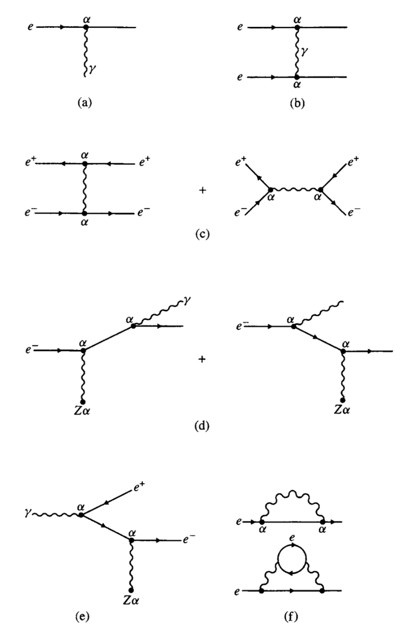
Feynman diagrams for QED — Fig. 4.1 Example Feynman diagrams for the QED interactions#

A combination of more than one of these vertexes is needed to describe a physical process. Diagram (b) shows the QED interaction between two electrons via the exchange of a “virtual” photon. The matrix element for each of the vertexes is proportional to \(\sqrt{\alpha}\), hence the matrix element \(\mathcal{M}_{f i}\) is proportional to \(\alpha\). The virtual photon introduces a propagator factor (discussed in the previous section) proportional to \(1 / q^{2}\) ( \(q\) is the momentum transferred in the process, e.g. the momentum of the photon). So the matrix element is proportional to

(4.1)#\[ \begin{equation*} \mathcal{M}_{f i} \propto \frac{\alpha}{q^{2}} \end{equation*} \]

And the cross section is then proportional to

(4.2)#\[ \begin{equation*} \sigma \propto\left|\mathcal{M}_{f i}\right|^{2} \propto \frac{\alpha^{2}}{q^{4}} \end{equation*} \]

Which leads to the formula for the Rutherford scattering with a charge to the power of 4 at the numerator and the fourth power of the momentum transfer at the denominator. In Fig. 4.1, the factor \(\alpha\) associated to each vertex, refers to the square of the matrix element term, e.g. the factor that we get in the cross section formula.

Diagram (c ) shows the diagrams for the interaction of an electron and a positron. Two different diagram, with a different time orientation, are needed to describe this process with (slightly) different calculations needed.

Diagram (d) describes the phenomenon of Bremsstrahlung, which is the emission of a photon from an electron in interaction with a nuclear field. While diagram (e) shows how the process \(\gamma \rightarrow e^{+} e^{-}\)that can take place in presence of a nuclear field. Note that neither process (d) or (e) are allowed in vacuum, and can only take place in the presence of an external nuclear field. As you can see in the diagram the external electric field of the nucleus interacts via the exchange of a photon.

Diagrams under (f) represent self-interaction terms. These are characteristic of a quantum field theory and require a bit more discussion, which we will cover in the next section.

4.2. Charged particles precession in a magnetic field - Classical treatment#

There are several properties which exhibit the quantum nature of the electromagnetic interaction. One of these is the magnetic moment of charged leptons, in particular the muon. We will see how QED can predict the magnetic momentum of a muon with a precision of about one part per million.

Before we study the quantum phenomenon, let’s look at a spinning charged particle in a magnetic field and show how a precession is observed in classical electromagnetism. We consider a particle of mass \(m\) and charge \(Q\), as shown in Fig. 4.2.

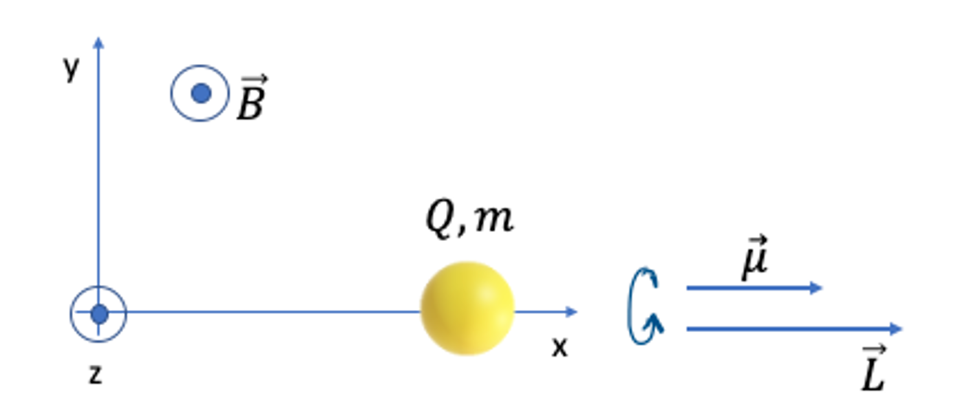
magnetic spin of a muon — Fig. 4.2 Spinning particle of mass \(m\) and charge \(Q\) in a magnetic field \(B\).#

This particle spins around the \(x\)-axis and, as a consequence, will carry an angular momentum \(\vec{L}\). Since the particle is charged, we have a charge distribution moving, and as a consequence a magnetic moment \(\vec{\mu}\). Under the assumption that mass and charge are uniformly distributed, we can say that \(\vec{\mu}\) and \(\vec{L}\) are parallel and in the \(x\)-direction.

In electromagnetism the ratio between the magnetic moment and the angular momentum is called the gyromagnetic ratio and it can be shown that

\[ \begin{equation*} \gamma_{\mathrm{gm}}=\frac{\mu}{L}=\frac{Q}{2 m} \end{equation*} \]

We should stress that this result is valid in the non-quantum mechanical situation. The magnetic moment interacts with the magnetic field \(\vec{B}\) resulting in a torque given by

\[ \begin{equation*} \vec{\tau}=\vec{\mu} \times \vec{B} \end{equation*} \]

in the configuration of Fig. 4.2 the torque points in the \(y\)-direction and is perpendicular to the angular momentum \(\vec{L}\). Since the torque is equal to the derivative of the angular momentum, the angular momentum magnitude does not change, while its direction rotates. This results in a gyroscopic motion of the charge, similar to what is experienced in a mechanical gyroscope. The precession frequency of the gyroscope is given by

\[ \begin{equation*} \omega_{P}=\gamma_{\mathrm{gm}} B \end{equation*} \]

4.3. Quantum field treatment of a particle with spin#

In the quantum case, the equivalent of a particle rotating around its axis is the spin of the particle itself. The calculation of the gyromagnetic ratio needs to be done using the rules of QED and leads to

\[ \begin{equation*} \gamma_{\mathrm{gm}}=g \frac{\mu_{B}}{\hbar} \end{equation*} \]

where \(\mu_{B}=e \hbar / 2 m\) is the Bohr magneton defined in your atomic physics course, and \(g\) is a constant that depends on the particle considered. You should note that for \(g=1\) we find the classical value calculated in the previous section.

In the case of the charged leptons, the calculation of \(g\) is performed using QED rules. In the following we consider a \(\mu^{+}\) particle for simplicity, and we will show how the value calculated from theory compares with the experimental value. You may have seen in the news that is a measurement that is performed with ever increasing precision and is a field of current research.

From a QED point of view, the muon interacts with the magnetic field through the exchange of a “quantum” of the field, a photon as in the diagram of Fig. 4.3.

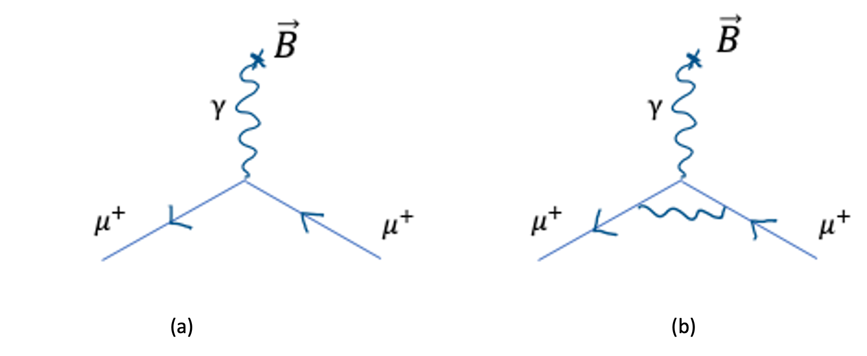
Feynman diagram of muon-B interactons — Fig. 4.3 Feynman diagrams for the interaction of a muon in a magnetic field. The diagram (a) corresponds to the leading order contribution, while (b) is a higher order contribution.#

The calculation of the leading order diagram on the left leads to \(g=2\) for electrons and muons. This leads to the precession frequency

\[ \begin{equation*} \omega_{P}=\gamma_{\mathrm{gm}} B=g \frac{e \hbar}{2 m} B=\frac{g}{2} \frac{e}{m} B \end{equation*} \]

An experiment can be conducted putting in a magnetic field muons with a velocity \(v\), polarised in a direction perpendicular to the field itself. The muons will travel along a circular trajectory in this magnetic field due to the Lorentz force with a rotation frequency of

\[ \begin{equation*} \omega_{R}=\frac{e}{m} B \end{equation*} \]

In the case \(g=2\), the two frequencies are the same, which means that the angle between the polarisation and the direction of travel of the muon remains constant. However the situation in QED is more complicated as other Feynman diagrams need to be calculated to take into account diagrams with more vertexes than the original one. An example of such diagram is shown in Fig. 4.3 (b) with a closed loop on the bottom part of the diagram. Since this diagram has more vertexes, its contribution to the matrix element will be proportional to a higher power of the fine structure constant \(\alpha\) and will lead to a slight modification of the value of \(g\), which is measured to be about 0.1% larger than 2. A full QED calculation, involving thousands of diagrams gives a theoretical value of \(g\) as

\[ \begin{equation*} g_{\mu}=2.0023318418(13) \end{equation*} \]

With an uncertainty of one part per billion. A pretty precise number! And a great challenge for both experimental and theoretical physicists to achieve this level of precision in their measurement and calculations.

4.4. Experimental measurement of g-2#

A pioneering experiment to measure \(\mathrm{g}-2\) for the muon was performed by a team including the late Prof. Combley of this department. A polarised beam of muons was circulated in a circular orbit in a uniform magnetic field. The quantity measured is the deviation from 2 defined as

\[ \begin{equation*} a=\frac{g-2}{2} \tag{120} \end{equation*} \]

The actual polarisation of the muons was measured through their parity nonconserving weak decays, \(\mu^{+} \rightarrow e^{+} \bar{\nu}_{\mu} \nu_{e}\). This process is mediated by a \(W\) boson (as will be discussed in the section of the course on weak interactions), and it can easily be shown, by considering the helicities of the neutrino and antineutrino, that, in the rest frame of the \(\mu^{+}\), the direction of decay of the \(e^{+}\) preferentially follows the direction of the muon’s spin. In the laboratory frame, the highest energy electrons have their decay momentum parallel to the muon’s momentum, and this information can be used to measure the spin of the muons before they decay. Exploiting these facts, the precession rate, and so the value of \(a\), were measured.

The results from the original 1981 experiment at CERN show an agreement of the experimental and theoretical value of \(a\) to a few part per million:

\[\begin{split} \begin{aligned} \text { Experimentally: } & a=(1165924 \pm 9) \times 10^{-9} \\ \text { QEDcalculation } & a=(1165921 \pm 8) \times 10^{-9} \end{aligned} \end{split}\]

In 2001, a similar experiment at Brookhaven compared more precise experimental results with better theoretical calculations - incorporating higher order Feynman diagrams - and tantalisingly found a 3 standard deviation discrepancy. This could be due to the existence of undiscovered particles beyond the standard model of particle physics. A third-generation experiment at Fermilab is ongoing in an attempt to elucidate the situation, having achieved a precision of 0.43 ppm . The size of the discrepancy got larger, however that called into question the validity of the theoretical calculations with different approaches from different groups obtaining different results. The investigation is still ongoing and is a current question if new physics is hiding behind a measurement with a precision better than a part per million.

Example 4.1 Muon decay lifetime

In the \(g-2\) experiment muon circulate in a ring of radius \(R=7.112\) m and an energy \(E=3.096\) GeV. The lifetime of the muon in the rest-frame is \(\tau = 2.197\ \mu\)s and the mass of the muon is \(m=105.7\) MeV. Calculate the average number of loops the muon do before decaying.

4.5. Further material#

Interactions, Feynman diagrams and the Yukawa potential can be found in Sections 1.4 and 1.5 of [Martin];
The whole QED topic is covered in sections 2.1, 2.2, 2.3, 2.4 and 2.5 of [Perkins]
The g-2 measurement is discussed in [Perkins] Section 2.5
A simplified explanation of the \(g-2\) experiment at Fermilab and its statistical implications can be found at the Fermilab web page https://muon-g2.fnal.gov/. The seven minutes video linked in the webpage is particularly useful.
A full review of the \(g-2\) measurement is available in Nucl. Phys. B 975 (2022) 115675. Link: https://www.sciencedirect.com/science/article/pii/S0550321322000268
A vintage (fun?) video from the 1960s at CERN explaining the first \(g-2\) experiment: https://www.youtube.com/watch?v=0bPV4HJrvlc
The original paper \(g-2\) paper, Phys. Rep. 68 (1981) 93-119, is available at http://cds.cern.ch/record/134110